Introduction
Locating fiber cable problems can be a real challenge for a technician! Before accessing a cable, some important things may need considering:
- Is the situation all an initial install, or is (some of) the link in service?
- Is another route available to take traffic while the link is being worked on?
- Is the fault a break interrupting service, or just a known loss point that ought to be investigated and fixed?
- Access to the cables: Can you walk along the route and inspect it, is it in ducts, on overhead poles or direct buried in the ground?
- How long is the route, 100 meters or 100 Km?
- Cabling type.
- What sort of fault locator is readily available.
- Who is available, with which skills?
You would be very well advised to spend some time experimenting with fault finding techniques for your application. This will avoid having to experiment on a live system, which may cause further damage to both the system, and your reputation.
The biggest problems with fault finding are
- Without disrupting a link, it may be impossible to measure a transmission signal. Can any connected transmission equipment show power levels?
- Non-metallic cables can be very hard to locate. A standard metallic locating device won't work on all-dielectric cables. Unfortunately, there is no such thing as a "fiber optic" locater, so to overcome this, it is common practice to bury some sort of metallic marker nearby these cables for location purposes.
- Route lengths can be very long, e.g. 100 Km. That’s a long way to go looking for a tree root!
- These systems are quite reliable, so people often have little fault-finding experience when it does go wrong.
- These links are often high capacity, high value, and need restoring now (no kidding), and that last working pair must not be disturbed.
- Because this is a relatively new technology, much of the gear and work practices related to maintenance are changing and are poorly understood.
- Skilled staff may not be available.
Some fault location techniques are:
- An OTDR (optical time domain reflectometer) is basically an optical radar that send a pulse up the line and analyses the echo. OTDRs are good at examining long links, up to 100 Km or more. This instrument is really useful to tell you that there is a problem, and to give a good idea of its approximate location. However, when you get to the fault area, it may not give sufficient detail to actually locate the fault. Developed as long-range instruments, they are often not so useful on short links, due to dead zone effects.
- A visible fault locator is a fiber optic laser light tester that can be used to find problems and check continuity over lengths of only a few Km. It can also be used along with an OTDR tester to find a fault with greater accuracy.
- A clip-on identifier is not strictly a fault locator, but is included here because it is often used during fault location to avoid disturbing working systems. It can be used to help actively find a fault, since it can show presence / absence of traffic or a test tone at a point, however this requires access to patch leads, or joint re-entry.
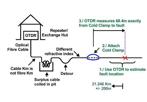
- Kingfisher’s unique Cold Clamp can be used in conjunction with OTDRs on jelly filled cables. It works by providing a local physical and optical reference marker which can be positioned near the fault site. The exact distance from the Cold Clamp to the fault can be measured on the instrument, and then physically measured on the ground. Long distance fault location with 1 m accuracy can be regularly achieved in this way.
Visible fault location
This technique was pioneered using Helium-neon lasers producing red light at 628 nm. As a laser light for fiber testing, this worked well, however the lasers used often had a short life and were very bulky. Kingfisher International developed & sold the first commercial semiconductor VFL in 1992. These 670 nm devices were gradually replaced by brighter units at 650 nm, and 635 nm.
The evolving laser wavelength is important because of the human eye (photopic) response, which is much better at 635 nm than at 670 nm. Maximum power level is limited by eye laser safety considerations to below +10 dBm (Laser Class 2M), so the lack of response at 670 nm cannot be compensated by boosting the power available. At the same power level 635 nm devices appear 8 times (9 dB) brighter than the old 670 nm types.
Companies trying to sell the older 670 and 650 nm lasers emphasize that they are visible further along the link than the newer types, since they are attenuated less rapidly. However, for most users the argument is usually spurious, since performance becomes increasingly erratic at these longer distances, making some other method more reliable in practice.
At Kingfisher we have experimented with green lasers, but these were found to be not very useful for various reasons to do with the fiber and cable.
It seems that 650 / 635 nm will remain the optimal wavelengths for this application, regardless of future advances in lasers.
Use of visible fault locators is dependent on many conditions and attempts to define them as having a particular distance range are fairly pointless. However, the maximum possible distance over which some light can be seen emerging from a cleaved end, is about 10 Km for 670 nm, and rather less for 635 nm. This is only useful if you are actually looking at ends!
A common use of visible fault locators is to locate a problem or break in a patch box or cables within an exchange. The break shows as a bright red light shining through the side of the sheath. Of course, the ability to do this depends on the light being able to get through the sheath. Many 3 mm patch lead cables readily allow the light through, however some colors (particularly purple and black) seem to be opaque to red light, and may not show anything.
It is better to verify expected performance with a visible fault locator before proceeding. It is even better to take this into account when specifying the cables in the first place.
A common use of visible fault locators in the LAN environments is to check continuity and duplex connector polarity.
Another useful function is the ability to see if light can get to a particular point on a link. To do this, put a sharp bend into the fibre, and visible light may leak out of the side of the sheath. It may be appropriate to shield as much ambient light as possible while doing this: maybe cover yourself with a ground sheet.
Visible fault locators are also extremely handy for finding problems with installed splitters and active devices. Without this technique, there is often very little alternative to dismantling a coupler assembly to find a suspected problem. Using visible fault location, it is often possible to find a fault with minimal disturbance.
Visible fault locators can also be used to rescue patch leads that have one faulty connector. The faulty connector will often glow brightly when light is injected into it.
Clip On Identifiers
A clip on identifier is clamped onto a patch lead to determine if there is a tone present, or traffic or nothing. This requires access to the fibers or patch cables, and a bit of slack to allow some bending.
Readings may be adversely affected by colored plastic coatings absorbing the light.
Identifiers should be tested for the amount of increased loss they create, since this can drop out live systems. They tend not to give totally reliable results and are often affected by stray light.
For these reasons, they should be used only to verify the link status before disconnection. They are preferably not used indiscriminately to locate a one of many possible active fibers. They are, however, a lot better than nothing!
Finding Faults on MPO Cables
Cables with multi-fiber MPO connectors are a new challenge for the fiber optic industry. Commonly they are used on very short links, with pre-assembled onto the cable. Typical problems include continuity, polarity, and dirt.
Kingfisher has developed the easy & versatile MPO Visual Cable Verifier to assist with these situations.
OTDRs for fault finding
Optical time domain reflectometers send a powerful laser pulse up a link and analyse the reflections. The reflected signal is very weak and may require extensive averaging to reduce detection noise. The user has to input information such as refractive index, pulse length and link length. From this, the OTDR calculates the reflected power level at each point, and from this, it is possible to determine loss figures, the location of point losses, and length.
In order to work over a range of applications, the emitted pulse length can be varied as in the chart below. A long (high energy) pulse gives long range or fast acquisition, a nice smooth output (ideal for commissioning), but very poor distance resolution (bad for fault location). So longer pulse lengths are used for longer links, or installation certification. Short (low energy) pulses give best distance resolution, but a noisier signal, and can only work at low attenuation levels. Short pulses may require a lot of averaging to get a good signal, which may take some minutes. So shorter pulse are used for fault location.
OTDRs have some theoretical difficulty with point losses, or reflections, in that the mathematics doesn't work very well at that point. The point loss or reflection is actually located by the intersection of the characteristics each side of it, eg by further deduction. There will also be some practical difficulty with point losses or reflections, in that the high gain detector amplifier may saturate or become slew-rate limited, creating a blind spot immediately after the event. This is called the dead-zone and is a genuine limitation. The dead-zone is also pulse length dependent. The theoretically calculated dead zone is shown in the table.
| Pulse length |
Dead zone |
| 1 nsec |
0.15 m (theoretically) |
| 10 nsec |
1.5 m (theoretically) |
| 100 nsec |
15 m |
| 1 µsec |
150 m |
| 10 µsec |
1.5 Km |
| 100 µsec |
15 Km |
In practice, some older instruments have a minimum dead-zone of 50 meters, and more modern units have a minimum of 2 - 10 metres on the shortest pulse lengths. Also, some modern units automatically change the pulse length as the unit searches further up the link. This is obviously highly desirable.
It should also be noted that dead-zone specification is with a mated, low-reflective PC type connector. In multimode systems, the connectors are highly reflective, so longer dead zones are observed than in the instrument data sheet. This is universal in the industry, and is not the fault of one manufacturer.
OTDRs were developed for long range applications over many Km on telecom style links. Effectiveness on short or multimode systems of under a Km in length is questionable, since dead zone effects mean that it is often impossible to differentiate one loss point (e.g. connector), from another. It is often impossible to do much fault location in this type of situation. This problem is often not understood by system designers, who insist on OTDR certification on a 100 metre run. The problem ends up as this: you need the highest performance instruments, in a situation where it is of the least possible value.
Another example of this problem is with modern PON applications. An "FTTX" OTDR may have a very short deadzone specification, however to see through the loss of a 32 way splitter requires a pulse length of 1 - 10 µsec, in which case the actual deadzone is between 150 - 1,500 meters, which is not very useful on a short distance PON.
The mathematical deduction process can also lead to some peculiar effects: some splices and connectors can appear to have optical gain. This happens when joined sections have slightly different characteristics, and the second section has a higher level of intrinsic back scatter than the first. However, if the same joint is measured from the opposite direction, the loss will appear abnormally high. This anomaly is solved by performing the measurement in both directions, and then averaging the result.
From all this, it should be apparent that for fault finding, the user must be careful to optimize both distance and amplitude resolution for a particular situation, and that the job will be slower than certification.
The noise reduction achievable by signal averaging is limited by the square root of the sample time. Therefore, each time signal averaging is extended by a factor of 4, a 3 dB increase in range is obtained. This creates a practical limit, for example extending a 10 minute average (fairly boring) to 1 hour (really boring), only yields a 4 dB increase in range. However, increasing from 1 second to 10 minutes, yields a 14 dB improvement!
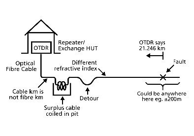
Limitations of using an OTDR by itself
Under ideal conditions the distance uncertainty of an OTDR is about ± 1%, e.g. 20 meters per Km. Some causes of this are:
- Even under factory conditions, the accuracy of cable length markers is about ± 0.5%. By the time cables are laid, this is likely to get worse.
- There is some variation in the ‘take up factor’, e.g. the fiber / cable length ratio. Due to this variation, experts regard length markers as the most accurate length measurement. Variations in ‘take up factor’ directly affect the accuracy of length measurement.
- The refractive index may vary along a route. It is often measured & specified to only 3 decimal places. Not all data will be totally accurate, not all installers record it accurately, and not all OTDRs can accept multiple values. Variations in refractive index directly affect the accuracy of length measurement.
- Link length may not match the route distance due to excess being coiled and left in pits, or undocumented detours.
- The exact route may also not be precisely mapped or followed. Minor discrepancies that would not be noticed during construction & acceptance, can cause havoc during precise fault location.
In practice, these uncertainties do matter, and where the cause of a fault is hidden (e.g. ground movement, tree roots, rocks, rodents etc), locating the loss point using OTDRs sometimes takes man days of work, and creates a network hazard while 100 meters or more of cable is unearthed.
Cold Clamp fault location
The Cold Clamp is a unique device developed by Kingfisher which overcomes some of the fundamental limitations of OTDRs.
The Cold Clamp works on jelly filled cables as typically used in long distance links, by acting as both a local physical and optical reference point.
A Cold clamp is attached to the cable close to the estimated fault location, but far enough away to avoid dead-zone problems. Liquid nitrogen is poured into the Cold Clamp, which creates a temporary optical loss point of approximately 0.2 - 1 dB. This can be used as a localized reference marker which can be picked up on the OTDR. It’s distance from the fault is measured with the OTDR cursors, and then it’s physical distance to the fault is measured on the ground.
OSP crews who have used the system find uses for it in all manner of situations where they would like to know a position accurately. For example, during installation, to mark known danger points on the route, such as rivers, roads, other cables etc.
Case history
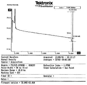
A link was partially broken. An ORDR trace showed a break at 4.2779 Km. The route map showed this as close to a river crossing. During a mobile phone conversation, the site crew remembered that there had been problems at the river crossing before, so they were pretty sure they knew that the problem was at the river crossing. However, the engineer in charge decided to check with a Cold Clamp.
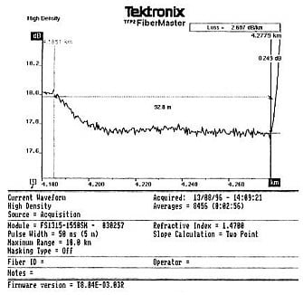
The line was excavated, and a Cold Clamp applied at a convenient point about 40 metres from the river. A trace as per Fig 11.2 was obtained, showing in general terms the break, and Cold Clamp loss point. The picture was zoomed in and the trace in Fig 11.3 obtained. This clearly showed the loss induced by the Cold Clamp at 4.185 Km and the break at 4.2779 Km. Moving the cursors to the start of each event showed 92.8 meters.
This was surprising, since this was in fact 50 meters away from the expected fault site at the river crossing. There was the inevitable discussion between the crew who thought they knew from past experience where the fault was to be found, and the measurement crew who disagreed with them. In the end, the measurement crew prevailed, the distance was measured out on the ground, and excavation revealed a fracture "within a shovel width" of the predicted location. It turned out that the construction crew had bogged a D9 dozer at the exact point of the fault.
Use of the Cold Clamp in this instance saved hours of work trying to find a fault in the wrong place, with all the extra network hazard that this would have entailed.
Particular points about this incident
This was an experienced repair crew, with accurate maps, route data and other aids. They had prior knowledge of the route. It was practically the ‘ideal’ situation. Despite all this, the fault was in a different place to that expected. The fault would of course have been located and fixed in time, however use of the Cold Clamp markedly improved the on-site processes, reduced costs & improved service provision.